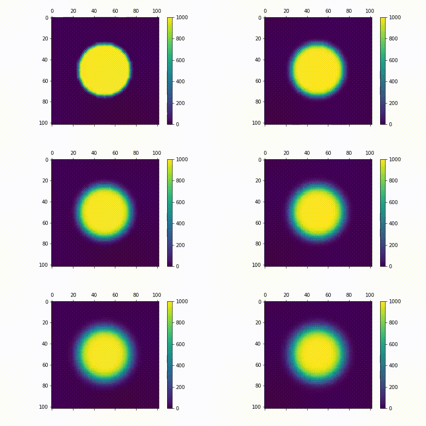
A Discrete Diffusion Process
05 Oct 2020 |python CUDA numba The goal of this post is to simulate a discrete diffusion process. We're going to do this with a regular CPU serial programming implementation, and then accelerate and parallelise with Numba.
Problem Statement
We are given a 2-dimensional grid with points $(i,j)$, such that $i,j\in {1,\dots, N }$, and start with an initial distribution $u_0 (i,j)$ of function valus on the grid points. The distribution process follows the following recurrence relation:
$$ u_{n+1}(i,j) = \frac{1}{4}[u_n(i+1, j) + u_n(i-1, j) + u_n(i, j+1) + u_n(i, j-1)] $$
The following boundary conditions are also applied:
- $ u_n(i, 0) = u_0(i, 0) $
- $ u_n(i, N+1) = u_0(i, N+1) $
- $ u_n(0, j) = u_0(0, j) $
- $ u_n(N+1, j) = u_0(N+1, j) $
CPU Code
The way this will work is we can evaluate the entire grid for a single diffusion step. Then, we can call this function for each iteration we wish to have. Here's the function:
CPU Code
import numpy as np

### Regular Python Function ###

def diffusion_iteration(un):
    """
    Perform one diffusion step for all given grid points.

    Parameters
    ----------
    un : numpy.ndarray
        Numpy array of type `float64` and dimension (N + 2, N + 2) that stores the
        function values at step n.

    This function returns a Numpy array of dimension (N + 2, N + 2) of type `float64`
    that contains the function values after performing one step of the above diffusion
    iteration.
    """

    n = np.shape(un)[0] - 2 # we set n = (N + 2) - 2 = N
    result = np.copy(un)

    ## Distribution Process for each cell not on the boundary
    for i in range(1,n+1):    # Note: indices range from 1 to n to exclude the boundary cells
        for j in range(1,n+1):
            # Taking the average of the four surrounding grid points
            result[i,j] = (un[i+1, j] + un[i-1, j] + un[i, j+1] + un[i, j-1])/4

    return result
The function is straight forward but obviously it will take a long time if $N$ is big. I think this function's time-complexity is $O (N^2)$, so run time will increase exponentially with $N$.
Accelerating with Numba
We can accelerate our previous function so that it can handle larger values of $N$. This is still a serial programming implementation, but at least it will be faster. We can do this with the @njit decorator, and the rest of the function will be the same.
Numba Serial Programming
from numba import njit, prange

### Serial Numba Implementation ###
    ## The only difference with this function is the addition of @njit decorator

@njit
def diffusion_iteration1(un):
    """
    Perform one diffusion step for all given grid points.

    Parameters
    ----------
    un : numpy.ndarray
        Numpy array of type `float64` and dimension (N + 2, N + 2) that stores the
        function values at step n.

    This function returns a Numpy array of dimension (N + 2, N + 2) of type `float64`
    that contains the function values after performing one step of the above diffusion
    iteration.
    """

    n = np.shape(un)[0] - 2 # we set n = (N + 2) - 2 = N
    result = np.copy(un)

    ## Distribution Process for each cell not on the boundary
    for i in range(1,n+1):    # Note: indices range from 1 to n to exclude the boundary cells
        for j in range(1,n+1):
            result[i,j] = (un[i+1, j] + un[i-1, j] + un[i, j+1] + un[i, j-1])/4
            # Taking the average of the four surrounding grid points

    return result
Parallelise with Numba
The Numba accelerated implementation is better than the regular serial implementation, but we can make it run faster still. We can parallelise the computations using Numba's prange function in the outermost loop.
Parallel Numba Programming
## Parallel Numba Implementation

@njit(['float64[:,:](float64[:,:])'], parallel = True)
def diffusion_iteration2(un):
    """
    Perform one diffusion step for all given grid points.

    Parameters
    ----------
    un : numpy.ndarray
        Numpy array of type `float64` and dimension (N + 2, N + 2) that stores the
        function values at step n.

    This function returns a Numpy array of dimension (N + 2, N + 2) of type `float64`
    that contains the function values after performing one step of the above diffusion
    iteration.
    """

    n = np.shape(un)[0] - 2 # we set n = (N + 2) - 2 = N
    result = np.copy(un)

    ## Distribution Process for each cell not on the boundary
    for i in prange(1,n+1):    # Note: indices range from 1 to n to exclude the boundary cells
        for j in range(1,n+1):
            result[i,j] = (un[i+1, j] + un[i-1, j] + un[i, j+1] + un[i, j-1])/4
            # Taking the average of the four surrounding grid points

    return result
Visualisation
Here's a visualisation for the diffusion process. I used $N=100$. For my initial distribution $u_{0} (i,j)$, I have points within a central circle with radius $r=25$ to have values 1000 (i.e $u_{0} (i,j)= 1000 $ if $i, j \in \{ (i,j) \mathrel{} | \mathrel{} i^2 + j^2 \leq 625 \}$ )
