Heating a Square Plate
20 Nov 2020 |python CUDA numba Problem Statement
We will consider a square plate with sides \( \left[ -1,1 \right] \times \left[ -1,1 \right]\). We have the following initial conditions at time $t=0$:
- The temperature of 3 sides is $u_0=0$.
- The temperature of the fourth side is $u_0=5$.
We would like to find time \( t = t^{'} \) such that \( u(t^{'}) = 1 \) at the center of the plate.
We are given the correct time \(t^{'} = 0.424011387033 \).
To do this, we will implement a finite difference scheme with both forward and backward time-stepping.
Solution
First, we note that the temperature of the plate obeys the heat equation: $$ \frac{\partial u}{\partial t} = \alpha \Delta u $$ where $\Delta$ is the standard Laplacian operator (we work in coordinates \( {x, y, t}\)). Furthermore, \( \alpha \) is some positive coefficient of the medium. We will use \( \alpha = 1\) for simplicity.
We denote \( u(x,y,t) = u_{i,j}^{k}\) where \( i, j\) represent the spatial coordinates and \(k\) represents the time-step.
We can solve this problem using two different implementations: a forward Euler method (both CPU and GPU) and a backward Euler method (CPU).
Implementation 1 - Forward Euler Method
The forward difference is given by
$$ \frac{du}{dx} \approx \frac{u_{i+1} - u_{i}}{h} $$
Further, second-order derivatives are approximated by:
$$ \frac{d}{dx} \left [\frac{d}{dx} u \right] = \frac{u_{i+1} - 2u_{i} - u_{i-1}}{h^2} $$
Applying these two relations to the heat equation, we get:
$$ \frac{u_{i,j}^{k+1} - u_{i,j}^{k}}{\Delta t} = (\frac{u_{i+1,j}^{k} - 2u_{i,j}^{k} - u_{i-1,j}^{k}}{h^2} + \frac{u_{i,j+1}^{k} - 2u_{i,j}^{k} - u_{i,j-1}^{k}}{h^2}) $$
where $\Delta t$ is the discretized time step, and $h$ is our discretized spatial step. We are able to obtain our final equation:
$$ u_{i,j}^{k+1} = (1-4C)u_{i,j}^{k} + C(u_{i+1,j}^{k} + u_{i-1,j}^{k} + u_{i,j+1}^{k} + u_{i,j-1}^{k}) $$
where \( C = \frac{\Delta t}{h^2} \).
This method is stable if: \( \Delta t \leq \frac{h^2}{4} \).
A CPU Implementation
First we have a standard CPU computing method for the Euler forward method. We have used NUMBA's parallel processing to accelerate the performance.
CPU Code
def initialize(N, iterations):
    """
    Creates the initial array for the plate
    ---
    N = plate size
    iterations: number of time steps
    """
    #Initializaing the plate
    plate = np.zeros((iterations, N, N))
    plate[ :, N-1, :] = 5

    return plate

@njit
def forward_step(plate, N, iterations):
    """
    Performs forward euler method
    ----
    plate = array representing the temperatures of the plate
    N = plate dimensions (spatial)
    iterations = number of time-steps we wish to perform
    """

    alpha = 1
    h = 2/(N-1)
    time_step = (h**2)/(4*alpha)
    C = time_step/(h**2)

    middle = (N-1)//2
    result_time = 0
    for k in prange(0, iterations-1):
      for i in range(1, N-1):
        for j in range(1,N-1):
            if plate[k, middle, middle] >= 1.0:
                result_time = k
                print('CPU Iterations: ', result_time)
                return result_time
            plate[k+1, i, j] = (1-4*C)*(plate[k, i,j]) + C*(plate[ k, i+1, j] + plate[ k, i-1, j] + plate[ k, i, j+1] + plate[ k, i, j-1])

    return 999
Initializing the plate and running forward_step will let us evaluate this implementation.
A GPU Implementation
We also present a GPU computing method for the Euler forward scheme. The CPU controls each time-step iteration, while the GPU performs the computation of the square plate for each time-step.
GPU Code
## Our GPU Kernel ##
@cuda.jit
def gpu_forward(N, input_array, C, result_array):
    ## Shared Memory Arrays ##
    shared = cuda.shared.array((34, 34), numba.float32)

    ## Positioning - Local ##
    tx = cuda.threadIdx.x
    ty = cuda.threadIdx.y

    ## Positioning - Global ##
    px, py = cuda.grid(2)
    index = (N-2)*py + px

    if px >= N-2:
        return
    if py >= N-2:
        return

    ## Loading data into shared memory ##
    # Middle
    shared[tx+1, ty+1] = input_array[(N-2)*py + px]

    # Filling in the edges
    if px == 0:
        shared[tx, ty+1] = 0
    if px == N-3:
        shared[tx+2, ty+1] = 0
    if py == 0:
        shared[tx+1, ty] = 0
    if py == N-3:
        shared[tx+1, ty+2] = 5

    if (tx == 0) and (px != 0):
        shared[tx,ty+1] = input_array[(N-2)*py + px - 1]
    if (tx == 31) and (px != N-3):
        shared[tx+2, ty+1] = input_array[(N-2)*py + px + 1]
    if (ty == 0) and (py != 0):
        shared[tx+1, ty] = input_array[(N-2)*(py-1) + px]
    if (ty == 31) and (py != N-3):
        shared[tx+1, ty+2] = input_array[(N-2)*(py+1) + px]

    # Sync Threads
    cuda.syncthreads()

    ## Performing Stencil ##
    if index < (N-2)**2:
        stencil = (1-4*C)*shared[tx+1,ty+1] + C*(shared[tx,ty+1] + shared[tx+2,ty+1] + shared[tx+1,ty] + shared[tx+1,ty+2])
        result_array[index] = stencil

        # Sync Threads
        cuda.syncthreads()


## A function to help evaluate the GPU kernel ##
def eval_gpu_forward(gpu_plate, N, iterations):
    """
    Create initial array and evaluates GPU Euler forward step
    """
    SX = 32
    SY = 32
    nblocks = (N + SX - 1) // SX
    blockspergrid = (nblocks, nblocks)
    threadsperblock = (SX, SY)

    middle = (N-1)//2

    for k in range(0, iterations-1):
        gpu_prev_plate = gpu_plate[k, 1:(N-1), 1:(N-1)].reshape((N-2)**2)
        gpu_result = np.zeros((N-2)**2, dtype = np.float32)

        gpu_forward[blockspergrid, threadsperblock](N, gpu_prev_plate, C, gpu_result)
        gpu_plate[k+1, 1:(N-1), 1:(N-1)] = gpu_result.reshape((N-2), (N-2))

        if gpu_plate[k+1, middle, middle] >= 1.0:
            gpu_time = k + 1
            print('GPU Iterations: ', gpu_time)
            return gpu_plate[k+1, :, :], gpu_time

    print('The center never reached u = 1')
    return gpu_plate[k,:,:], 999999999999
Initializing the plate and running eval_gpu_forward will let us evaluate this implementation.
Implementation 2: Backward Euler Method
The backward difference is given by:
$$ \frac{du}{dx} \approx \frac{u_{i} - u_{i-1}}{h} $$
Further, second-order derivatives are approximated by:
$$ \frac{d}{dx} \left [\frac{d}{dx} u \right] = \frac{u_{i+1} - 2u_{i} + u_{i-1}}{h^2} $$
Applying these two relations to the heat equation, we get:
$$ \frac{u_{i,j}^{k} - u_{i,j}^{k-1}}{\Delta t} = (\frac{u_{i+1,j}^{k} - 2u_{i,j}^{k} + u_{i-1,j}^{k}}{h^2} + \frac{u_{i,j+1}^{k} - 2u_{i,j}^{k} + u_{i,j-1}^{k}}{h^2}) $$
Therefore, we get our final equation of
$$ u_{i,j}^{k-1} = (1 + 4C) u_{i,j}^{k} - C (u_{i+1,j}^{k} + u_{i-1,j}^{k} + u_{i,j+1}^{k} + u_{i,j-1}^{k} ) $$
where \( C = \frac{\Delta t}{h^2} \).
We note that this method is unconditionally stable.
Unlike the forward method, we cannot use this equation alone. We note that we may express the same equation as a time-dependent matrix equation:
$$ u^{k-1} = A u^{k} $$
Then applying the inverse matrix on both sides, we get:
$$ A^{-1} u^{k-1} = u^{k} $$
A CPU Implementation
In this implementation, we require that we generate the sparse matrix A. We solve the matrix equation using spsolve in every time iteration to find the next configuration of the plate.
CPU Code
def generate_inverse(N):
    nelements = 5 * N**2 - 16 * N + 16

    row_ind = np.empty(nelements, dtype=np.float64)
    col_ind = np.empty(nelements, dtype=np.float64)
    data = np.empty(nelements, dtype=np.float64)

    f = np.empty(N * N, dtype=np.float64)

    alpha = 1
    h = 2/(N-1)
    time_step = (h**2)/(4*alpha)
    C = time_step/(h**2)

    count = 0
    for j in range(N):
        for i in range(N):
            if i == 0 or i == N - 1 or j == 0 or j == N - 1:
                row_ind[count] = col_ind[count] = j * N + i
                data[count] =  1
                f[j * N + i] = 0
                count += 1

            else:
                row_ind[count : count + 5] = j * N + i
                col_ind[count] = j * N + i
                col_ind[count + 1] = j * N + i + 1
                col_ind[count + 2] = j * N + i - 1
                col_ind[count + 3] = (j + 1) * N + i
                col_ind[count + 4] = (j - 1) * N + i

                data[count] = 1 + 4*C
                data[count + 1 : count + 5] = - C
                f[j * N + i] = 1

                count += 5

    return coo_matrix((data, (row_ind, col_ind)), shape=(N**2, N**2)).tocsr()

def cpu_backward(backward_plate, N, iterations):
    cpu_prev_plate = backward_plate[0, :, :].reshape(N**2)
    A = generate_inverse(N)

    for k in range(iterations - 1):
        sol = spsolve(A, backward_plate[k, :, :].reshape(N*N))
        backward_plate[k+1, :, :] = sol.reshape((N,N))

        if (backward_plate[k+1, middle, middle] >= 1) and (backward_plate[k, middle, middle] < 1):
            print("Iterations: ", k+1)
            cpu_back_time = k+1

            return backward_plate[k, :, :], cpu_back_time
Initializing the plate and running cpu_backward will let us evaluate this implementation.
Note: We have set $h = \frac{2}{(N-1)} $ in all of our implementation methods. This is because our plate must have edges which take points $[-1, 1]$. Therefore, our choice of $h$ is to ensure that each side of our plate has length 2.
Validation
These are the errors I got for all three implementations:
Euler Forward (CPU) Error: 7.053204587920749e-05
Euler Forward (GPU) Error: 7.053204587920749e-05
Euler Backward (CPU) Error: 0.0004890281047001464
These errors are pretty negligible. For the forward methods, I got up to $N = 181$, but for the backward method I only managed to get to $N=81$. This is because the backward method is significantly more time-consuming, but answers why the backward method had a much higher error.
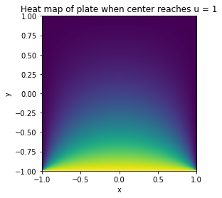
Visualization
It might be interesting to visualise the heat dynamics of the plate when the center point reaches $u(t') = 1$. All three methods yielded the same image: